
Plan the investigation
What does gravity-only motion look like?
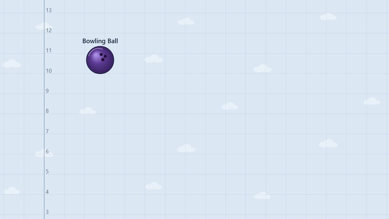
In ideal free fall, the only force acting on the object is gravity. The prepared scene starts a Bowling Ball about 10.7 m above the ground with an initial vertical velocity near zero. With up chosen as positive, the gravitational acceleration is ay = −9.8 m/s².
Change or control
Control release height, initial vertical velocity, and gravitational field strength. Keep air resistance off so the gravity-only model remains clear.
Measure and compare
Record y, vy, and ay at equal times. Use the slope of y–t to find vertical velocity, the slope of vy–t to find acceleration, and the signed vy–t area to find vertical displacement.
A negative vy means downward motion. A negative ay means the acceleration points downward; it does not mean the object must already be moving downward.
Procedure
A useful five-trial workflow
- Load and inspect. Launch the simulation and choose Free Fall. Select the Bowling Ball in Objects, open Properties, and record its starting y position, mass, and initial vy. Open Data → Graph; the prepared scene starts with vertical position selected.
- Set the sign convention. Keep up as positive and gravity near −9.8 m/s². Leave air resistance and applied forces off. If you want a visual direction check, turn on the acceleration vector after recording the starting state.
- Predict and run. For a drop from rest, use Δy = ½ay(Δt)² and vy = ayΔt. Run for about 1.0 s before contact and record the same time rows in every trial.
- Analyze one graph at a time. Display y, vy, and ay separately. The y–t curve should be concave down, the vy–t line should have slope −9.8 m/s², and the ay–t line should be horizontal at −9.8 m/s².
- Change one condition and repeat. Reset before changing release height or initial vy. Compare predicted and measured values, then use Export CSV for the full motion history. Stop a trial before the ball contacts the ground when analyzing the gravity-only model.
| t (s) | Δy (m) | vy (m/s) | ay (m/s²) |
|---|---|---|---|
| 0.00 | 0.00 | 0.00 | −9.80 |
| 0.25 | −0.31 | −2.45 | −9.80 |
| 0.50 | −1.23 | −4.90 | −9.80 |
| 0.75 | −2.76 | −7.35 | −9.80 |
| 1.00 | −4.90 | −9.80 | −9.80 |
The prepared ball starts close to 10 m above its contact point, so the ideal impact time is about 1.43 s and the impact speed is about 14.0 m/s downward. Contact with the ground ends the gravity-only portion of the trial.
Worked example
Predict a drop from rest
Use a rounded drop distance of 10.0 m, viy = 0.00 m/s, and ay = −9.80 m/s².
0 = Δy = viyt + ½ayt² = 0.00 − 4.90t²
timpact = √(2h/g) = √(20.0/9.80) = 1.43 s
vfy = ayt = −9.80(1.43) ≈ −14.0 m/s
The position graph bends downward because its slope becomes more negative. The velocity graph falls in a straight line, and the acceleration graph stays constant. The area under vy–t from release to impact gives the negative drop distance.
Expected data pattern
Use the three graphs as cross-checks
For the rounded drop model, the ideal values below should agree with the displayed Data rows before contact. Small differences come from the exact starting height, ball radius, and simulation time step.
| t (s) | y change (m) | vy (m/s) | ay (m/s²) | Graph check |
|---|---|---|---|---|
| 0.00 | 0.00 | 0.00 | −9.80 | release |
| 0.50 | −1.23 | −4.90 | −9.80 | speed increasing downward |
| 1.00 | −4.90 | −9.80 | −9.80 | linear vy slope |
| 1.43 | −10.00 | −14.0 | −9.80 | near impact |
A slope measurement on y–t gives vy at that instant. A slope measurement on vy–t gives ay. The horizontal ay line is evidence that the acceleration is constant.
Common misconception
Free fall is about the forces, not just the direction of motion
An object is in ideal free fall when gravity is the only force controlling it. It can be moving up, moving down, or momentarily stopped.
At the highest point of an upward throw, is acceleration zero?
No. vy is zero for an instant, but ay remains −9.8 m/s².
Does a heavier object fall faster in this model?
No. Mass changes the weight force, but the ratio of weight to mass gives the same gravitational acceleration when air resistance is ignored.
Is every falling object in free fall?
No. A parachute, a supported elevator passenger, or an object with a significant drag force has forces besides gravity acting on it.
For teachers
Compare drops, throws, and models
Have students predict the signs of y, vy, and ay before running. Then compare the position graph’s concavity with the velocity graph’s slope and the acceleration graph’s level.
Extend the investigation with an upward launch. At the apex, students should identify vy = 0 while acceleration remains downward, then use the symmetry of the ideal trajectory to compare the time up and time back to the launch height.
Use the mass-comparison trial to show that equal gravitational acceleration does not mean equal weight. The Constant Acceleration lab generalizes the same graph relationships, while the Projectile-Motion Independence lab applies free-fall reasoning to vertical motion inside a two-dimensional launch.
Reference guides: Free Fall Motion and Acceleration Graphs.