
Core idea
Use slope, height, and area for different quantities
A velocity–time graph reports velocity at each instant. Its slope is acceleration: a rising line means positive acceleration, a falling line means negative acceleration, and a horizontal line means zero acceleration even when the object is moving quickly.
An acceleration–time graph reports acceleration directly. The area under the curve gives the change in velocity. An area above the time axis increases velocity; an area below the axis decreases it. A position–time graph completes the chain because its slope is velocity and its concavity shows whether that slope is increasing or decreasing.
Read the vertical axis first
Graph height only has meaning after you identify the plotted quantity. A high velocity is not automatically a high acceleration, and a high position is not automatically a high speed.
Follow the graph chain
Slope of x–t gives v. Slope of v–t gives a. Area under the v–t curve gives displacement, and area under the a–t curve gives Δv.
Guided lesson path
Build the graph hierarchy from one motion
- Start with a changing position slope. Run from v0 = +1.0 m/s with a = +2.0 m/s². The x–t graph gets progressively steeper because velocity increases.
- Measure velocity-graph slope. Display only vx and measure its slope. From v = 1.0 m/s at 0 s to v = 5.0 m/s at 2 s, the slope is +2.0 m/s².
- Use area under the curve. The vx–t trapezoid from 0 to 2 s has area 6.0 m, while the ax–t rectangle has area 4.0 m/s. These give displacement and velocity change.
- Read a multiflash record. Compare four segments with positive acceleration, zero acceleration, negative acceleration, and zero acceleration. Equal-time spacing grows, stays wide, shrinks, then stays closer together.
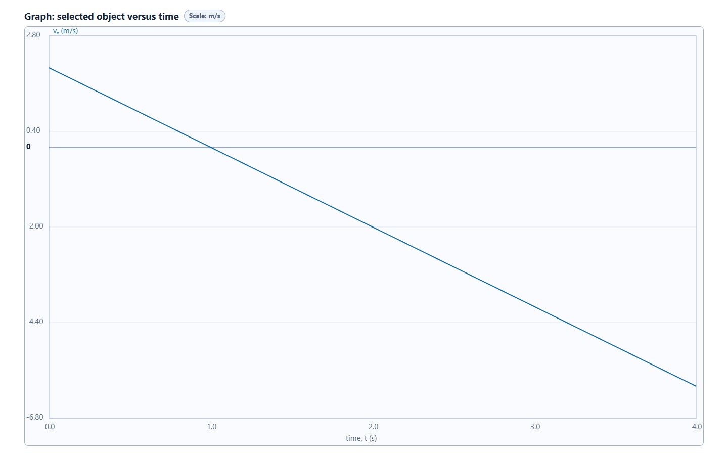
- Analyze reversal and concavity. Use x0 = 3 m, v0 = +2 m/s, and a = −2 m/s². The object moves right, stops at 1 s, reverses, and produces a concave-down position graph.
| Time interval | Acceleration | Velocity behavior | Equal-time spacing |
|---|---|---|---|
| 0–2 s | +1.5 m/s² | Increases from +0.5 to +3.5 m/s | Grows |
| 2–4 s | 0 m/s² | Constant at +3.5 m/s | Equal and wide |
| 4–5 s | −2.5 m/s² | Decreases to +1.0 m/s | Shrinks |
| 5–7 s | 0 m/s² | Constant at +1.0 m/s | Equal and closer |
The velocity graph rises, stays flat, falls, and stays flat again. The acceleration graph records the matching sequence: positive, zero, negative, zero.
Worked examples
Connect graph measurements to equations
For the first trial, velocity rises from 1.0 m/s to 5.0 m/s in 2.0 s:
a = slope of v–t = (5.0 − 1.0)/2.0 = +2.0 m/s²
The velocity graph forms a trapezoid with parallel sides 1.0 m/s and 5.0 m/s:
Δx = area under the curve = ((1.0 + 5.0)/2)(2.0) = +6.0 m
The acceleration graph is a +2.0 m/s² rectangle for 2.0 s:
Δv = area under the curve = (2.0)(2.0) = +4.0 m/s
Graph relationships
Translate among x–t, v–t, and a–t
| Graph | Read directly | Operation |
|---|---|---|
| x–t | Position from height | Slope = velocity; concavity reveals acceleration sign |
| vx–t | Velocity from height | Slope = acceleration; area under the curve = displacement |
| ax–t | Acceleration from height | Area under the curve = change in velocity |
For the reversal trial with x0 = 3 m, v0 = +2 m/s, and a = −2 m/s², the whole four-second motion has vf = −6 m/s and xf = −5 m. The velocity area is +1 m before the turn and −9 m after it, giving Δx = −8 m.
Position-graph shape
Concavity shows how velocity changes
A position graph can rise while curving downward. That means velocity is still positive, but its slope is becoming less positive because acceleration is negative. When the slope reaches zero, the object is momentarily at rest; if the curve continues downward, the velocity becomes negative and the object reverses.
Positive acceleration makes an x–t graph concave up, negative acceleration makes it concave down, and zero acceleration produces a straight segment. The graph’s vertical intercept is initial position, so changing x0 shifts the curve without changing its slope pattern or concavity.
Common misconceptions
Check the reasoning
Is acceleration the height of a velocity graph?
No. Acceleration is the slope of the velocity–time graph. A horizontal velocity line above zero has positive velocity and zero acceleration.
Does positive velocity guarantee positive acceleration?
No. An object can move right while slowing down, so velocity is positive while acceleration is negative.
Does a rising position graph always mean positive acceleration?
No. Rising means positive velocity. If the curve is concave down, the positive velocity is decreasing and acceleration is negative.
Does area below the axis represent negative distance?
No. Area under a signed velocity curve gives signed displacement. Distance remains a nonnegative path length; the negative sign records motion toward decreasing position.
For teachers
Ask students to name the operation
Before each graph interaction, have students identify the vertical-axis quantity and predict whether slope, area under the curve, height, or concavity is the relevant evidence.
Use the reversal trial to separate three ideas that are often blended together: a positive position slope, a negative acceleration, and a concave-down curve can all occur at the same time. Then ask students to verify the endpoint displacement from the velocity graph area.
Continue with the Constant Acceleration Simulation and Virtual Lab, review slope and area with Position and Velocity Graphs, and connect the graph chain to Free Fall Motion. The prepared experiment page supplies the interactive starting scene.