
Core idea
Acceleration is a rate, not a velocity
Constant acceleration means that velocity changes by the same amount during equal time intervals. If a = +5.0 m/s², the velocity increases by 5.0 m/s every second. The object can be speeding up, slowing down, or reversing; the acceleration is still constant as long as that rate of velocity change stays fixed.
Position responds to the changing velocity. During equal time intervals, the object generally travels different distances because it enters each later interval with a different velocity. That is why a nonzero constant acceleration produces a curved position–time graph even though the acceleration–time graph is horizontal.
Track the signs
Choose +x before running. Velocity and acceleration point in the same direction when speed increases and in opposite directions when speed decreases. A positive acceleration does not automatically mean speeding up.
Read the graph chain
The slope of x–t is v, the slope of v–t is a, and the signed area under v–t is Δx. The area under a–t gives Δv.
Guided lesson path
A useful five-trial workflow
- Observe a baseline. Run the prepared traveler with vi = +2.0 m/s and a = +5.0 m/s². Watch velocity change while the acceleration vector stays constant.
- Build acceleration. Use Set acceleration to create a +4.0 m/s² vector, then compare its one-second velocity change with the +5.0 m/s² trial.
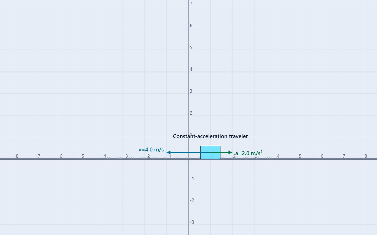
- Compare directions. Run vi = −4.0 m/s with a = +2.0 m/s². The traveler moves left while slowing, reaches v = 0, and then reverses to the right.
- Analyze one graph at a time. Display vx–t and measure its slope. Display ax–t to see the constant value, then display x–t to connect increasing slope with increasing velocity.
- Test scaling. Use the equations and graph areas to predict displacement, then compare stopping trials at 35 m/s and 70 m/s with the same braking acceleration.
| t (s) | x (m) | vx (m/s) | ax (m/s²) |
|---|---|---|---|
| 0.0 | 0.0 | +2.0 | +5.0 |
| 1.0 | 4.5 | +7.0 | +5.0 |
| 2.0 | 14.0 | +12.0 | +5.0 |
| 3.0 | 28.5 | +17.0 | +5.0 |
The velocity changes by +5.0 m/s in every one-second interval, while the one-second displacements are 4.5 m, 9.5 m, and 14.5 m. Equal velocity changes do not create equal position changes.
Worked examples
Choose the equation that matches the known quantities
For the baseline trial after 2.0 s:
vf = vi + aΔt = 2.0 + (5.0)(2.0) = 12.0 m/s
Δx = viΔt + ½a(Δt)² = (2.0)(2.0) + ½(5.0)(2.0)² = 14.0 m
If the lesson starts from rest with a = +10.0 m/s² for 2.0 s, the v–t graph rises from 0 to 20 m/s. Its triangular area is 20 m, which matches the displacement equation.
When elapsed time is not known, use vf² = vi² + 2aΔx. For a vehicle braking from 35 m/s at −15 m/s²:
Δxstop = (0² − 35²)/(2·−15) = 40.83 m
Graph reading
Use slope and area as evidence
| Graph | Read from it | Constant-acceleration shape |
|---|---|---|
| x–t | Slope gives v | Curved when a is nonzero; slope changes steadily |
| vx–t | Slope gives a; signed area gives Δx | Straight line with slope a |
| ax–t | Signed area gives Δv | Horizontal line at the constant acceleration |
Keep one series visible while using Slope or Area. A graph can look simple while still carrying a different physical quantity: the height of x is position, the slope of x is velocity, and the area under v is displacement.
Proportional reasoning
Why doubling speed quadruples stopping distance
For a fixed braking acceleration, stopping occurs when vf = 0. Rearranging the no-time equation gives Δxstop = vi²/(2|a|). The square on initial speed is the key relationship.
| Initial speed | Braking acceleration | Stopping time | Stopping distance |
|---|---|---|---|
| 35 m/s | −15 m/s² | 2.33 s | 40.83 m |
| 70 m/s | −15 m/s² | 4.67 s | 163.33 m |
| 35 m/s | −30 m/s² | 1.17 s | 20.42 m |
Doubling speed multiplies stopping distance by four. Doubling the magnitude of braking acceleration cuts stopping distance in half. The simulation lets you test both predictions with the same measurement method.
Common misconceptions
Check the reasoning
Does constant acceleration mean constant velocity?
No. Constant acceleration means velocity changes at a constant rate. Constant velocity requires zero acceleration.
Does positive acceleration always mean speeding up?
No. With v = −4.0 m/s and a = +2.0 m/s², the vectors point in opposite directions, so the object slows until it reverses.
Is acceleration zero when velocity is zero?
No. At a reversal, velocity is zero for an instant while the nonzero acceleration continues to change it.
Does a negative acceleration always mean slowing down?
No. If velocity is also negative, the vectors point in the same direction and the object speeds up toward negative x.
For teachers
Move from vectors to equations to graphs
Ask students to predict the vector directions before running each trial. Have them state whether speed should increase or decrease, then use the vx–t slope to verify the acceleration sign.
For a graph-centered assessment, hide force arrows, show only one data series, and require students to report both a slope or area and the matching kinematics equation. The stopping-distance trials provide a concrete proportional-reasoning check that is easy to compare across groups.
Continue with the Constant Acceleration Simulation and Virtual Lab, then connect the same vertical model to Free Fall Motion and graph relationships to Acceleration Graphs. The editable lab documents are available from the experiment page.