
Plan the investigation
What does constant velocity look like?
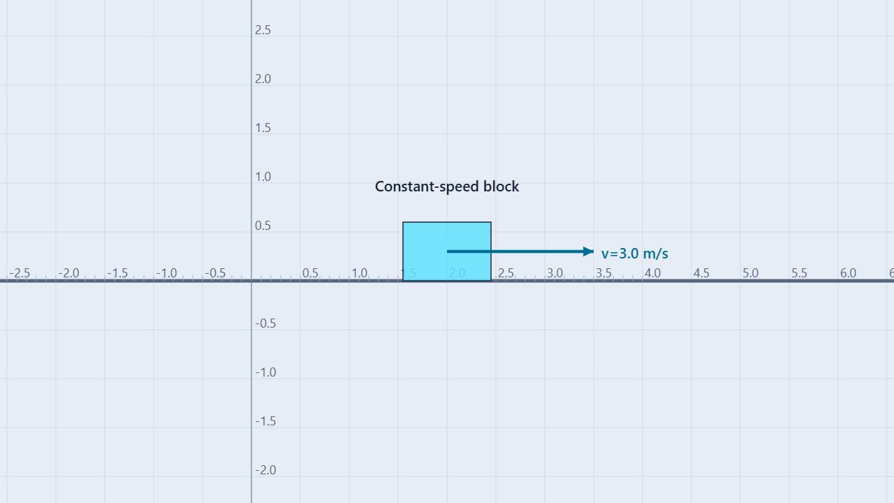
In one-dimensional motion, constant speed and constant velocity are the same only when the direction does not change. The prepared Constant Speed scene starts a block at x = 2.00 m with vx = +3.00 m/s on an infinite frictionless surface. Gravity and the normal force balance vertically, so the horizontal velocity stays unchanged.
Change
Set the block’s initial x velocity to −4, −2, 0, +2, and +4 m/s. Keep its initial position, y velocity, surface, and gravity fixed.
Measure
Record x, vx, and ax at the same times. Use the x–t slope to find velocity and the signed area under vx–t to find displacement.
Choose a sign convention before you run: positive x points right. A negative velocity means motion toward decreasing x; it does not mean that the object has negative speed.
Procedure
A useful five-trial workflow
- Load and inspect. Launch the simulation and choose Constant speed from the experiment menu. Select the Constant-speed block in Objects, open Properties, and record its starting x position and x velocity.
- Set one velocity. Reset the trial, edit the block’s initial x velocity, and keep y velocity at 0 m/s. Use the five values in the table below. Leave the frictionless surface and gravity unchanged.
- Predict and run. Predict x after 2.00 s using x = x0 + vxt. Set a 2-second run duration beside Play, then run from t = 0.
- Analyze one graph at a time. Open Data → Graph and display x, vx, and ax. Keep only one series visible while using Inspect or Slope. The x–t slope should equal vx; the vx–t line should be horizontal; and ax should remain zero.
- Compare and preserve evidence. Reset before each new velocity. Record the same time rows for every trial, compare measured values with the predictions, and use Export CSV if you need the complete sample history.
| vx (m/s) | x at 1.00 s (m) | x at 2.00 s (m) | Δx in 2.00 s (m) |
|---|---|---|---|
| −4.00 | −2.00 | −6.00 | −8.00 |
| −2.00 | 0.00 | −2.00 | −4.00 |
| 0.00 | 2.00 | 2.00 | 0.00 |
| +2.00 | 4.00 | 6.00 | +4.00 |
| +4.00 | 6.00 | 10.00 | +8.00 |
For every row, the position–time graph is a straight line. Changing velocity changes its slope; changing only x0 would move the line vertically without changing its slope.
Worked example
Read the prepared +3.00 m/s trial
The preset begins at x0 = 2.00 m and runs with vx = +3.00 m/s. After 2.00 s:
Δx = vxt = 3.00(2.00) = +6.00 m
x = x0 + Δx = 2.00 + 6.00 = 8.00 m
ax = Δvx/Δt = 0/2.00 = 0.00 m/s²
The x–t graph should rise with slope +3.00 m/s, the vx–t graph should stay at +3.00 m/s, and the ax–t graph should lie on zero. The block is moving even though its acceleration is zero.
Expected data pattern
Use equal-time rows as a check
For the unchanged +3.00 m/s preset, the ideal model gives these values. Use the displayed time in each Data row when comparing your own run; small rounding differences are expected.
| t (s) | x (m) | vx (m/s) | ax (m/s²) |
|---|---|---|---|
| 0.00 | 2.00 | +3.00 | 0.00 |
| 0.50 | 3.50 | +3.00 | 0.00 |
| 1.00 | 5.00 | +3.00 | 0.00 |
| 1.50 | 6.50 | +3.00 | 0.00 |
| 2.00 | 8.00 | +3.00 | 0.00 |
Use Slope on x versus t to recover the velocity. If you switch the graph’s horizontal axis to x, the vx line remains a useful measurement series but the slope question changes, so return to time before comparing trials.
Common misconception
Does zero acceleration mean zero velocity?
No. Zero acceleration means velocity is not changing. An object can move at a steady nonzero velocity, as the prepared block does.
Is constant speed the same as constant velocity?
Only when direction stays fixed. A car moving around a curve can keep constant speed while its velocity changes.
Does a negative position mean negative speed?
No. Position and velocity can carry signs; speed is the positive magnitude of velocity. A block traveling left at −2.00 m/s still has a speed of 2.00 m/s.
Does a higher position graph mean a faster object?
No. The height of an x–t graph gives position. Its slope gives velocity, so compare slopes rather than vertical intercepts.
For teachers
Connect motion, slope, and area
Have students sketch all three graphs before running. Ask them to explain why equal time intervals produce equal position changes, why the vx–t area equals displacement, and why the ax graph stays at zero.
Extend the investigation by comparing +2.00 m/s and −2.00 m/s. Their speed and displacement magnitudes over the same interval match, but their velocity signs and final positions differ. Then open the Constant Acceleration lab to see how a nonzero acceleration changes the graph shapes.
The Displacement and Velocity guide develops signed position changes, while the Position and Velocity Graphs guide focuses on slope and area. Physics reference: OpenStax, College Physics 2e, §2.4.