
Plan the investigation
How do motion diagrams and graphs tell two stories?
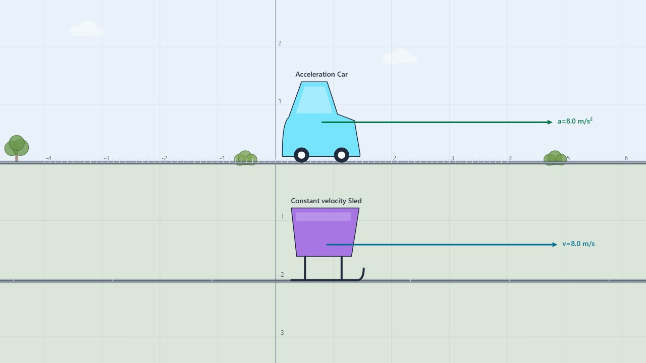
The prepared scene places a Constant velocity Sled beside an Acceleration Car. The sled moves at about +8.0 m/s with nearly zero horizontal acceleration. The car starts from rest with about +8.0 m/s² of horizontal acceleration. Both vehicles use the same ticker-tape interval, so their spacing can be compared directly.
Change or control
Keep the ticker-tape interval at 0.25 s for the first comparison. Then change one vehicle’s initial velocity or the car’s applied force while keeping the other starting conditions fixed.
Measure and compare
Compare dot spacing, x, vx, and ax. Use x–t slope to find velocity, vx–t slope to find acceleration, and the signed vx–t area to find displacement.
Use the same positive-x direction for both vehicles. Equal spacing means equal displacement during each equal time interval; growing spacing means the object is changing velocity.
Procedure
A useful five-trial workflow
- Load and identify. Launch the simulation and choose Motion Graphing: Constant Velocity and Acceleration. Confirm that the Constant velocity Sled and Acceleration Car are both present. Open Data → Graph and leave Ticker Tape Motion on.
- Predict before running. Sketch the dot spacing and the three graph shapes for each vehicle. Predict which object has a horizontal vx–t line and which has a sloped one.
- Run synchronized trials. Run for about 2.00 s. The 0.25 s ticker interval gives equal-time snapshots for both objects. Record the same time rows for the sled and car so the comparison is fair.
- Analyze one relationship at a time. Display x, vx, and ax in the graph workspace. Inspect x–t slopes for velocity, vx–t slopes for acceleration, and areas under vx–t for displacement. Hide extra series when a label or slope is hard to read.
- Change one condition and repeat. Reset, set the car’s acceleration to zero or give the sled a different initial velocity, and predict the new pattern. Export CSV when you need the full synchronized data set.
| t (s) | Sled Δx (m) | Sled vx (m/s) | Car Δx (m) | Car vx (m/s) |
|---|---|---|---|---|
| 0.00 | 0.00 | +8.00 | 0.00 | 0.00 |
| 0.50 | +4.00 | +8.00 | +1.00 | +4.00 |
| 1.00 | +8.00 | +8.00 | +4.00 | +8.00 |
| 1.50 | +12.00 | +8.00 | +9.00 | +12.00 |
| 2.00 | +16.00 | +8.00 | +16.00 | +16.00 |
The exact preset values may differ by a few hundredths because its prepared forces are tuned numerically. Use the displayed readings for evidence and the table for the ideal pattern.
Worked comparison
Compare the vehicles at 1.00 s
For the idealized trial, the sled keeps vx = +8.0 m/s, while the car starts from rest with ax = +8.0 m/s².
Sled: Δx = vt = 8.0(1.00) = +8.0 m, vx = +8.0 m/s, ax = 0.0 m/s²
Car: vx = vi + at = 0.0 + 8.0(1.00) = +8.0 m/s
Car: Δx = ½at² = ½(8.0)(1.00)² = +4.0 m
At that instant the vehicles have the same velocity but different displacements. The sled’s x–t graph is straight, the car’s x–t graph is curved, the sled’s vx–t graph is horizontal, and the car’s vx–t graph slopes upward.
Expected data pattern
Read the spacing and graph shapes together
Use these ideal values as a shape check. Your Data rows will include the vehicles’ absolute positions, while this table reports displacement from each starting position.
| t (s) | Sled ax (m/s²) | Car ax (m/s²) | Sled ticker spacing | Car ticker spacing |
|---|---|---|---|---|
| 0.00 | 0.00 | +8.00 | equal | — |
| 0.50 | 0.00 | +8.00 | equal | increasing |
| 1.00 | 0.00 | +8.00 | equal | increasing |
| 1.50 | 0.00 | +8.00 | equal | increasing |
| 2.00 | 0.00 | +8.00 | equal | increasing |
For the sled, equal ticker spacing and a horizontal vx–t graph agree. For the car, increasing spacing and a rising vx–t graph agree. In both cases, the ax–t graph is the fastest way to check whether acceleration is constant.
Common misconception
What does each graph actually tell you?
The vertical value of an x–t graph is position. Its slope is velocity. The slope of vx–t is acceleration, and its signed area is displacement.
Does equal ticker spacing mean the object is stopped?
No. Equal spacing means equal displacement during equal time intervals. A row of evenly spaced dots can represent a large constant velocity.
Does a horizontal velocity graph mean zero velocity?
No. It means velocity is constant. The line can sit at +8.0 m/s, −8.0 m/s, or zero.
Do the vehicles need to be side by side at the same position?
No. Compare their changes in position, velocities, and accelerations. Different starting positions shift an x–t graph vertically without changing its slope.
For teachers
Move from motion diagrams to calculus ideas
Ask students to describe each vehicle without using the words “fast” or “slow.” Require evidence from dot spacing, graph slope, and graph area. This keeps velocity, acceleration, and displacement distinct.
For an extension, set the car’s acceleration to zero and compare it with the sled. Then give the sled a negative initial velocity or give the car a negative acceleration. Students can predict when a velocity graph crosses zero and explain why a changing direction does not require a new coordinate system.
The Constant Speed lab isolates straight-line position graphs, while the Constant Acceleration lab develops equal velocity changes and kinematics equations. The Position and Velocity Graphs guide and Acceleration Graphs guide provide reference explanations.