
Plan the investigation
Hold torque fixed and change the mass distribution
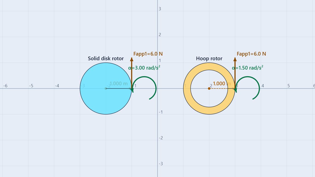
The prepared scene compares a solid disk and a thin hoop. Both have mass 4.00 kg, radius 1.00 m, and start from rest. Each receives the same 6.00 N upward tangential force at the rim. The centers are held in place so the comparison isolates rotation.
Keep fixed
Mass, radius, force magnitude, force direction, application point, and initial angular velocity.
Change one variable
Change the rotational-inertia factor or one controlled input, then reset before comparing the new trial with the baseline.
The disk and hoop have the same mass and size, but their mass is distributed differently relative to the axis. That difference changes I even though the applied force and lever arm are identical.
Build the model
Connect torque, inertia, and angular acceleration
For a force applied perpendicular to a radius, the torque magnitude is the force times the lever arm:
τ = r⊥F = (1.00 m)(6.00 N) = 6.00 N·m
Rotational inertia measures how strongly an object resists angular acceleration. In this simulation the inertia factor k sets the model I = kMR². A solid disk has k = 0.5; a thin hoop has k = 1.0.
Στ = Iα
I = kMR²
α = Στ/I
Because both rotors receive the same 6.00 N·m torque, the hoop’s doubled rotational inertia gives it half the angular acceleration of the disk. The force is not larger on the disk; the response is different because the mass distribution is different.
Procedure
Measure α and compare it with 1/I
- Load and inspect. Open Rotational Inertia Versus Angular Acceleration and select each rotor to record its mass, radius, inertia factor, and applied force.
- Check the control variables. Confirm both forces are 6.00 N, point upward at the 1.00 m rim, and produce the same positive torque. Confirm both angular velocities start at zero.
- Calculate before running. Use I = kMR² and α = τ/I to predict the angular acceleration of the disk and hoop.
- Run and collect evidence. Run the simulation briefly, pause it, and use the Data panel to inspect angular acceleration, angular velocity, and angle. The angular-velocity graph should have a slope equal to α while the torque is constant.
- Compare the rotors. Record at least three time samples for each object. Test whether the disk’s angular acceleration is about twice the hoop’s and whether αI stays close to the common torque.
- Change one factor. Reset, change only the inertia factor or the applied force, and repeat. State which relationship your new trial tests before you run it.
| Rotor | Inertia factor k | Rotational inertia I | Angular acceleration α | ω after 2.00 s |
|---|---|---|---|---|
| Solid disk | 0.50 | 2.00 kg·m² | 3.00 rad/s² | 6.00 rad/s |
| Thin hoop | 1.00 | 4.00 kg·m² | 1.50 rad/s² | 3.00 rad/s |
The simulator may display small numerical differences after stepping. Use values from the same paused frame and keep extra digits until the final comparison.
Worked example
Why the hoop accelerates more slowly
For the disk, the mass is closer to the axis on average:
Idisk = (0.5)(4.00)(1.00²) = 2.00 kg·m²
αdisk = 6.00/2.00 = 3.00 rad/s²
For the hoop, more of the mass is at the rim:
Ihoop = (1.0)(4.00)(1.00²) = 4.00 kg·m²
αhoop = 6.00/4.00 = 1.50 rad/s²
The hoop has twice the rotational inertia, so the same torque produces half the angular acceleration. If both start from rest and torque remains constant, ω = αt; after 2.00 s the disk should therefore have about twice the angular speed.
Compare trials
Use a controlled trial table
Keep the 4.00 kg mass, 1.00 m radius, and 6.00 N tangential force fixed while changing only the inertia factor. The predicted torque remains 6.00 N·m, so the product Iα should remain constant.
| Inertia factor k | I (kg·m²) | Predicted α (rad/s²) | Interpretation |
|---|---|---|---|
| 0.25 | 1.00 | 6.00 | Smallest I; fastest angular response |
| 0.50 | 2.00 | 3.00 | Solid-disk model |
| 0.75 | 3.00 | 2.00 | Intermediate mass distribution |
| 1.00 | 4.00 | 1.50 | Thin-hoop model |
Plot measured angular acceleration against 1/I. With torque held constant, the points should follow a straight-line relationship with slope equal to the applied torque.
Interpret the evidence
Read the slope of angular velocity
For constant torque and constant inertia, angular acceleration is constant. On an ω–t graph, the slope is α; on an angle–time graph, the curve becomes steeper because the angular speed is increasing.
slope of ω–t = α
α = Δω/Δt
τnet = Iα
Use the displayed torque, inertia, and acceleration from one trial to calculate a residual:
Rτ = τdisplayed − Iα
A small residual supports the rotational model. If it is large, check that the force is still applied at the rim, the rotor is not rotation-locked, and the values came from the same time sample.
Common misconceptions
Check the reasoning
Does the hoop receive less torque?
No. The baseline force and lever arm are the same, so both rotors receive about 6.00 N·m. The hoop accelerates less because its rotational inertia is larger.
Is rotational inertia just mass?
No. Rotational inertia depends on mass and how far that mass is distributed from the axis. Equal masses can have different values of I.
Does zero initial angular velocity mean zero angular acceleration?
No. The rotors start from rest, but the applied torque immediately produces angular acceleration.
Does a faster angular velocity prove a larger torque?
No. Angular velocity accumulates over time. Compare angular acceleration and torque at the same time before inferring a cause.
For teachers
Make the control variables visible
Require students to write the control variables before they run: equal mass, equal radius, equal tangential force, equal lever arm, and the same initial angular velocity. Then ask them to explain why the force vectors look the same while the angular-acceleration vectors differ.
Have students test both representations of the model: compare α for disk and hoop, then plot α versus 1/I across several inertia factors. A useful extension is to double the force while holding I fixed and predict that α doubles.
Review Newton’s Second Law, Work and Kinetic Energy, and Teeter-Totter Rotational Equilibrium. Physics reference: OpenStax, University Physics Volume 1, §10.4. Learn about the educator behind the simulations on the BuildPhysics About page.