
Plan the investigation
Does horizontal speed change flight time?
For an ideal projectile, horizontal launch velocity changes range but does not change flight time or maximum height when vertical launch velocity and the launch and landing heights stay fixed. Use five launches to test this prediction.
Change
Set horizontal velocity to 3, 5, 7, 9, and 11 m/s. Keep vertical velocity at +6.00 m/s and gravity at 9.80 m/s² downward.
Measure
Compare time to first landing, horizontal displacement, and the highest center position. Analyze the first flight, before any bounce.
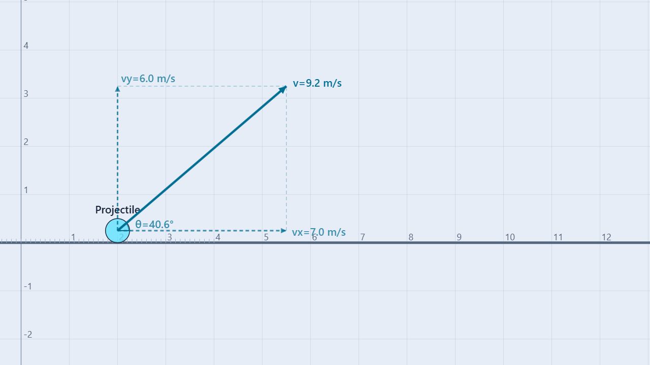
The preset ball has radius 0.25 m and starts with its center at x = 2.00 m, y = 0.25 m above a flat floor. Its center returns to y = 0.25 m at first contact. Treat the airborne motion as subject only to uniform gravity, with no air resistance or applied forces.
Procedure
A useful five-trial workflow
- Load the scene. Launch the simulation. If a saved scene appears, choose Projectile motion in the experiment menu. Open Properties and select Projectile in the Objects list.
- Set the launch. Expand Initial conditions. Under Velocity, enter the trial’s X value and keep Y at 6 m/s. Leave Position at X = 2 m and Y = 0.25 m. Check gravity in World and keep the ball’s radius unchanged.
- Predict and collect. Calculate range and flight time before running. Open the Data panel and choose Projectile as Object 1 in Graph. Enable x, y, and vᵧ. A 1.3 s run duration includes the first landing, predicted near 1.22 s.
- Identify first contact. Inspect the y graph for its first return to about 0.25 m and the vᵧ graph for the abrupt change at impact. Read x just before contact and subtract the starting x of 2.00 m to estimate range. Use Export CSV if you need the full sample history.
- Reset and repeat. Reset to the starting conditions before editing the next horizontal velocity. Compare all five trials. Explain why the y–time curves should overlap while the x–time slopes differ.
| v0x (m/s) | Flight time (s) | Range (m) | Rise above launch (m) |
|---|---|---|---|
| 3.00 | 1.224 | 3.673 | 1.837 |
| 5.00 | 1.224 | 6.122 | 1.837 |
| 7.00 | 1.224 | 8.571 | 1.837 |
| 9.00 | 1.224 | 11.020 | 1.837 |
| 11.00 | 1.224 | 13.469 | 1.837 |
Worked example
Predict the preset’s range, height, and flight time
Use v0x = 7.00 m/s, v0y = 6.00 m/s, and g = 9.80 m/s². Positive y points upward. At the peak, vy = 0:
tpeak = v0y/g = 6.00/9.80 = 0.612 s
Because the ball lands at the same center height at which it launched, its flight time is twice the time to the peak:
tflight = 2v0y/g = 12.00/9.80 = 1.224 s
R = v0xtflight = 7.00 × (12.00/9.80) = 8.571 m
Δymax = v0y²/(2g) = 36.00/19.60 = 1.837 m
The highest center position is 0.25 + 1.837 = 2.087 m. The predicted landing x is 2.00 + 8.571 = 10.571 m. Range is the change in x, not that final coordinate.
Simulation check
Read the rise and fall in the data
A run of the unchanged Projectile motion preset produced these airborne samples. The x position increases uniformly while vertical velocity passes from positive to negative near the top of the path.
| Time (s) | x (m) | y (m) | vy (m/s) |
|---|---|---|---|
| 0.500 | 5.500 | 2.025 | 1.100 |
| 0.600 | 6.200 | 2.086 | 0.120 |
| 0.700 | 6.900 | 2.049 | −0.860 |
| 0.800 | 7.600 | 1.914 | −1.840 |
At 0.500 s, the ideal equations give x = 2.00 + 7.00(0.500) = 5.500 m, y = 0.25 + 6.00(0.500) − 4.90(0.500)² = 2.025 m, and vy = 6.00 − 9.80(0.500) = 1.100 m/s. These agree with the displayed sample.
The Data panel samples at 30 Hz, so a recorded row need not coincide with the exact peak or first contact. Estimate those events between nearby samples. Do not use the later bounce to measure the original flight.
Common misconception
Is acceleration zero at the highest point?
No. Vertical velocity is momentarily zero, but vertical acceleration remains −9.80 m/s². The ball also retains its horizontal velocity, so its total speed at the peak is 7.00 m/s in the worked example.
Does a faster launch always mean more time in the air?
Increasing only the horizontal component does not lengthen the flight. Increasing the upward component does. State which component changes before making a prediction.
Does 45° always give the greatest range?
The 45° result assumes fixed launch speed, equal launch and landing heights, uniform gravity, and no air resistance. This investigation fixes the vertical component instead of total speed, so that angle comparison does not apply.
Can I use twice the time to the peak for a raised launch?
Only when landing and launch heights are equal. For different heights, solve ylanding = y0 + v0yt − ½gt² for the physical positive flight time, then use R = v0xt.
For teachers
Connect a trajectory to three time graphs
Ask students to sketch x–time, y–time, and vᵧ–time before running. Look for a straight x–time line, a curved y–time graph, and a straight vᵧ–time line with slope −g. A graph of range against horizontal launch velocity should have slope equal to flight time, about 1.224 s here.
Extend the investigation with the Projectile-Motion Independence lab, or use the Projectile Target Challenge to predict a landing point. Review the vertical motion in the Free Fall topic guide.
Physics reference: OpenStax, University Physics Volume 1, §4.3. Learn about the educator behind these simulations on the BuildPhysics About page.