
Plan the investigation
More force or more mass: what changes?
At fixed mass, doubling net force doubles acceleration. At fixed net force, doubling mass halves acceleration. Use two sets of trials to distinguish these relationships.
Investigation A: change force
Keep the block at 2.00 kg. Apply horizontal forces of 0, 3, 6, 9, and 12 N.
Investigation B: change mass
Keep the horizontal force at 6.00 N. Use masses of 1, 2, 3, 4, and 6 kg.
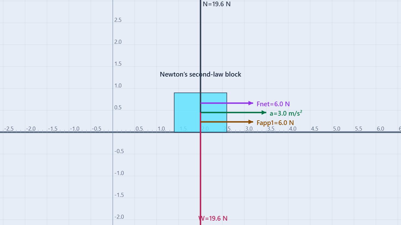
The prepared scene starts with a 2 kg block at rest and one 6 N force pointing right. The floor is horizontal and frictionless. Keep friction disabled, the applied force horizontal, and the block free to move. Positive x points right.
Draw three actual forces on the block: weight downward, normal force upward, and applied force to the right. Weight and normal force balance vertically. With no friction or other horizontal forces, ΣFx equals the applied horizontal force.
Read the forces
What accelerates the prepared block?
Vertical: ΣFy = 19.6 − 19.6 = 0 N
Horizontal: ΣFx = +6 N
Therefore: ax = +6/2 = +3 m/s²
Draw the actual forces first. Acceleration and net force summarize the result; they are not additional interactions to add to this diagram.
Procedure
A useful five-trial workflow
Use this workflow once for each investigation. Reset between trials so every run starts from rest.
- Load and inspect. Launch the simulation. If a saved scene appears, choose Newton’s second law from the experiment menu. Open Properties and select Newton’s second-law block in the Objects list.
- Set one variable. Edit Mass in Properties. Under Applied forces, edit Force 1’s x-component and leave its y-component at 0 N. For Investigation A keep mass at 2 kg; for Investigation B keep the x-component at 6 N.
- Predict and run. Calculate ax = ΣFx/m before pressing Play. Set the run duration beside Play to 0.5 seconds. Keep the initial velocity zero and all other settings unchanged.
- Read the evidence. Open the Data panel. The preset’s graph measurements are ΣFₓ, aₓ, and vₓ. Keep the block selected, then use the Data tab to record a sample at 0.300 s. In Graph, compare the vₓ–time slope with aₓ.
- Reset and compare. Reset the trial before entering the next value. Complete all five rows, then plot the measured acceleration against force for A and against reciprocal mass, 1/m, for B. Export CSV if you need the full sample history.
| ΣFx (N) | ax (m/s²) | vx at 0.500 s (m/s) |
|---|---|---|
| 0.00 | 0.00 | 0.00 |
| 3.00 | 1.50 | 0.75 |
| 6.00 | 3.00 | 1.50 |
| 9.00 | 4.50 | 2.25 |
| 12.00 | 6.00 | 3.00 |
| Mass (kg) | ax (m/s²) | vx at 0.500 s (m/s) |
|---|---|---|
| 1.00 | 6.00 | 3.00 |
| 2.00 | 3.00 | 1.50 |
| 3.00 | 2.00 | 1.00 |
| 4.00 | 1.50 | 0.75 |
| 6.00 | 1.00 | 0.50 |
Worked example
Predict the motion of the 2 kg block
For a constant horizontal net force of +6.00 N on a 2.00 kg block:
ax = ΣFx/m = 6.00 N / 2.00 kg = +3.00 m/s²
A newton is a kg·m/s², so dividing newtons by kilograms gives acceleration units. Starting from rest, after 0.500 s:
vx = v0x + axt = 0 + 3.00(0.500) = +1.50 m/s
Δx = v0xt + ½axt² = ½(3.00)(0.500)² = 0.375 m
The acceleration stays constant while velocity increases. Doubling both force and mass gives 12.00 N / 4.00 kg = 3.00 m/s², so that new pair produces the same acceleration.
Simulation check
Compare three observed runs
Three runs used the prepared frictionless scene, zero initial velocity, and a 0.5 s run duration. The rows below show readings at the same sampled time, 0.300 s. Only the stated mass or horizontal force changed from the baseline.
| Mass (kg) | ΣFx (N) | ax (m/s²) | vx (m/s) |
|---|---|---|---|
| 2.00 | 6.000 | 3.000 | 0.900 |
| 2.00 | 12.000 | 6.000 | 1.800 |
| 4.00 | 6.000 | 1.500 | 0.450 |
The readings match ax = ΣFx/m and vx = axt at the displayed precision. For the baseline, 3.00 × 0.300 = 0.900 m/s. The Data panel samples at 30 Hz; use the time printed in the row when checking a velocity prediction.
Common misconception
Does constant force mean constant speed?
A constant nonzero net force on a constant mass produces constant acceleration. Velocity changes continuously. Constant velocity requires zero net force.
Is the applied force always the net force?
No. They are equal horizontally in this frictionless, single-push setup. If a 2 N friction force opposes a 6 N push, the horizontal net force is 4 N; a 2 kg block then accelerates at 2 m/s².
Should I draw an extra “net force” arrow?
The net force is the vector sum of the actual forces, not another interaction. You may display it as a resultant, but do not add it again when calculating ΣF.
Does zero force stop a moving block?
Zero net force means zero acceleration. A block already moving on this ideal frictionless floor keeps its velocity. The zero-force trial stays at rest because its initial velocity is zero.
Make sense of the evidence
Use three graphs to check one prediction
Acceleration versus time
For the 2 kg, 6 N trial, expect a horizontal trace near +3 m/s² while the force remains constant and the block is free to move.
Velocity versus time
Expect a straight line starting at zero. Its slope, Δv/Δt, should agree with the measured acceleration.
Position versus time curves upward because the block covers more distance in each equal time interval. For motion from rest, Δx = ½at². A curved position graph is consistent with constant acceleration.
Check a velocity slope
For the ideal baseline, v at 0.100 s is 0.300 m/s and v at 0.400 s is 1.200 m/s. The predicted slope is (1.200 − 0.300)/(0.400 − 0.100) = 3.00 m/s². Repeat this calculation using two actual rows from your exported data and their printed times.
If your readings do not match
- Check that you selected the block rather than the floor or world totals.
- Confirm friction is disabled and Force 1 has no vertical component.
- Reset before editing the next trial so it starts from rest.
- Compare samples before any collision, and use acceleration rather than velocity when checking F/m.
Predict before you run
Can two different setups give the same acceleration?
Compare a 2 kg block with a 6 N push and a 4 kg block with a 12 N push. Predict the acceleration and velocity after 0.5 s for each, then test them.
Reveal the prediction and explanation
Both have F/m = 3 m/s². Starting from rest, both reach 1.5 m/s after 0.5 s and travel 0.375 m. Equal acceleration does not require equal force; it requires the same ratio of net force to mass.
Next, predict what changes if you reverse the force to −6 N on the 2 kg block. Explain the signs of acceleration and velocity rather than treating a negative value as an error.
Apply the same reasoning to the Modified Atwood Machine, where one hanging weight accelerates two masses, or the Inclined Plane, where only a component of gravity acts along the path.
For teachers
Use graph slopes to infer mass and force
For Investigation A, plot ax vertically against ΣFx horizontally. The slope is 1/m = 0.500 kg⁻¹. If you reverse the axes and plot force against acceleration, the slope is mass, 2.00 kg. State the axes before interpreting a slope.
For Investigation B, acceleration against mass is a curve. Plotting acceleration against 1/m makes a straight line with slope 6.00 N. Ask students to explain why doubling mass halves acceleration instead of subtracting a fixed amount.
As an extension, reset and apply −6 N to test direction, or predict the result of doubling both force and mass before running. Then apply the same reasoning to the Atwood Machine lab and identify which masses belong to that system.
Review the Free-Body Diagrams guide when separating actual forces from their sum. Physics reference: OpenStax, University Physics Volume 1, §5.3. Learn about the educator behind the simulations on the BuildPhysics About page.